14 Continuous Treatments
All methods in this book have been introduced using a binary treatment. A unit is either treated or untreated. A firm either receives a subsidy or does not. A municipality either opens a nursery school or does not. A region either crosses an eligibility threshold or does not.
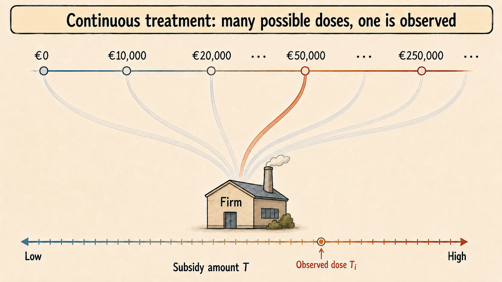
This binary representation is useful and often realistic. Policies may be organized around access—for example, receiving the program, being eligible for a benefit, or being exposed to a reform. In other settings, however, treatment is not simply a yes-or-no variable. Units may receive different amounts, intensities, or doses of the same policy.
For example, firms may receive different subsidy amounts. Regions may receive different amounts of EU Cohesion Policy funds per capita. Schools may receive different numbers of additional teachers. Patients may receive different drug dosages. Municipalities may experience different levels of exposure to an environmental shock.
In these cases, the question is not only whether the policy works. The question is also how the effect changes with the intensity of treatment.
With continuous treatments, causal inference studies how outcomes change as the dose or intensity of treatment changes.
14.1 From Binary Treatment to Treatment Intensity
In the binary case, each unit has two potential outcomes:
\[ Y_i(1) \quad \text{and} \quad Y_i(0). \]
With a continuous treatment, the treatment can take many values. Let \(T_i\) denote the treatment intensity received by unit \(i\). For each possible treatment level \(t\) within the relevant support of the treatment, unit \(i\) has a potential outcome:
\[ Y_i(t). \]
The observed outcome is
\[ Y_i^{obs}=Y_i(T_i). \]
As usual, we observe only one potential outcome for each unit: the one corresponding to the dose actually received. All other potential outcomes are counterfactual.
This is the continuous-treatment version of the fundamental problem of causal inference. The difference is that the missingness problem is now richer. Instead of missing one counterfactual outcome, we are missing the full schedule of potential outcomes over all treatment levels not received.
The relevant support of the treatment matters because causal effects can be studied only over treatment intensities that are meaningfully represented in the data. Extrapolating to doses that are rarely observed, or not observed at all, requires much stronger assumptions that are also inherently untestable.
14.2 Why Continuous Treatments Matter
Discretizing a continuous treatment into a binary variable can be convenient, but it often throws away important information.
Suppose a policy provides public subsidies to firms. A binary analysis compares subsidized firms with non-subsidized firms. This can answer whether access to the policy matters. But it cannot answer whether larger subsidies produce larger effects, whether the impact flattens after a certain amount, or whether low subsidies are too small to activate meaningful behavioral responses.
The same issue arises in regional policy. For instance, EU Cohesion Policy funds are allocated across regions classified as less developed, transition, and more developed. Yet funding intensity can remain highly heterogeneous even within the same category. Treating all supported regions as equally treated ignores potentially large differences in the amount of treatment received (Becker et al. 2012; Cerqua and Pellegrini 2018).
14.3 The Dose-Response Function
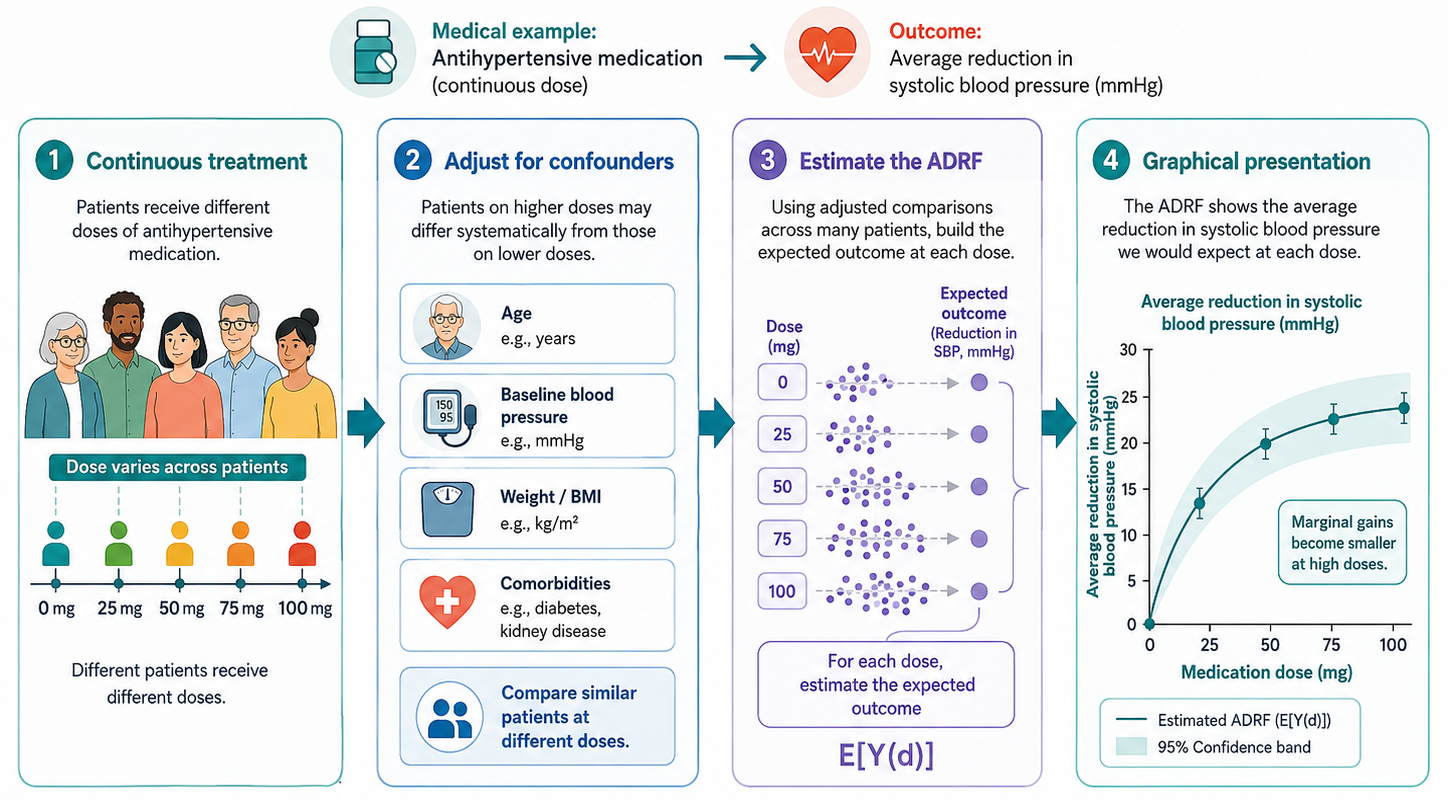
The main quantity of interest in continuous-treatment analysis is the average dose-response function (ADRF). It describes how the expected potential outcome changes with treatment intensity.
The ADRF is
\[ \mu(t)=E[Y_i(t)]. \]
For each treatment level \(t\), \(\mu(t)\) gives the average outcome that would be observed if all units received dose \(t\).
ADRF describes how the average potential outcome would change across different levels of treatment intensity. For each possible treatment level, it gives the average outcome that would be observed if all units were assigned that specific intensity.
The causal effect of increasing treatment from \(t_0\) to \(t_1\) can be written as
\[ \mu(t_1)-\mu(t_0). \]
If the treatment is continuous, we are usually also interested in the marginal effect of treatment intensity:
\[ \frac{\partial \mu(t)}{\partial t}. \]
This derivative describes how the expected outcome changes for a small increase in the dose.
The ADRF may be increasing, decreasing, flat, or nonlinear. For example, subsidies may increase firm employment at low levels of support but have little additional effect after a certain threshold. In that case, the policy may have diminishing returns.
14.4 The Policy Question
Continuous treatments shift the policy question from access to intensity.
With a binary treatment, we usually ask:
What is the effect of receiving the policy?
With a continuous treatment, we may instead ask:
What is the effect of receiving a larger dose of the policy? Is there an optimal level of treatment intensity?
This distinction has direct implications for policy design. If the ADRF flattens beyond a certain treatment intensity, allocating additional resources may yield only limited marginal returns. By contrast, if the ADRF continues to rise steeply, increasing treatment intensity may generate substantial additional benefits.
This chapter focuses on settings in which treatment varies continuously in intensity. A related challenge arises when treatment is discrete but has multiple versions. For instance, unemployed workers may participate in different active labor market programs, such as training, job-search assistance, or wage subsidies. In this setting, the relevant causal question is not simply whether receiving a program has an effect, but how the effects differ across alternative treatments.
The methods required for multiple discrete treatments differ from those used for continuous treatment intensity, even though both settings move beyond the standard binary treatment framework.1
1 Methods for multiple discrete treatments are not discussed in this book
14.5 The Challenge of Comparing Treatment Intensities
Continuous-treatment evaluation is difficult because treatment intensity is generally endogenous. Only when treatment intensity is randomly assigned can units receiving different doses be directly compared without further adjustment.
In most policies, however, the dose is not randomly assigned. Firms receiving larger subsidies may have larger projects, stronger administrative capacity, better political connections, or more severe constraints. Regions receiving more funds may differ systematically from those receiving less, as in the EU Cohesion Policy example. Patients receiving higher drug doses may have more severe baseline conditions.
Therefore, units receiving different treatment intensities are usually not directly comparable.
The fact that two units are both treated does not mean they are comparable. Units receiving different doses typically differ in ways that also affect their outcomes.
This is why, in observational studies, estimating an ADRF is not simply a matter of plotting outcomes against treatment intensity. A raw regression of \(Y_i\) on \(T_i\) compares different populations at different treatment levels. As a result, it may capture selection into dose rather than the causal effect of dose.
14.6 The Generalized Propensity Score
The propensity score was originally introduced for binary treatments (Rosenbaum and Rubin 1983), as shown in Chapter 5. Hirano and Imbens extended this idea to continuous treatments through the generalized propensity score, or GPS (Hirano and Imbens 2004).
In the binary case, the propensity score is the probability of receiving treatment conditional on covariates. In the continuous case, the GPS is the conditional density of the treatment level actually received:
\[ r(t,x)=f_{T\mid X}(t\mid x). \]
For unit \(i\), the GPS evaluated at the observed treatment level is
\[ R_i = r(T_i,X_i). \]
The GPS summarizes the likelihood of observing a given treatment intensity \(T_i\) for a unit with characteristics \(X_i\), as captured by the conditional density of treatment intensity given covariates.
The key result is that, under weak unconfoundedness (see below), adjusting for the GPS can help remove confounding due to observed covariates when estimating the ADRF.
14.6.1 Estimating the ADRF with GPS
Importantly, while a naive regression curve compares different units observed at different treatment levels, a GPS-adjusted ADRF aims to compare the same population under alternative treatment intensities. A typical GPS analysis proceeds in two stages.
First, estimate the treatment model. This means modeling the distribution of treatment intensity conditional on observed pre-treatment covariates:
\[ T_i \mid X_i. \]
In practice, this requires specifying a model for how treatment intensity is assigned. A common approach is to assume that, conditional on \(X_i\), the treatment follows a normal distribution:
\[ T_i \mid X_i \sim N(m(X_i),\sigma^2), \]
where \(m(X_i)\) is the expected treatment intensity given the covariates. The function \(m(X_i)\) can be estimated using a linear regression of \(T_i\) on \(X_i\), or with more flexible methods if the relationship between treatment intensity and covariates is expected to be non-linear. Once this model has been estimated, the GPS is obtained as the conditional density of the observed treatment level:
\[ \widehat{R}_i=\widehat{r}(T_i,X_i). \]
Second, estimate the outcome model. This means modeling the expected outcome as a function of both treatment intensity and the estimated GPS:
\[ E[Y_i \mid T_i=t, R_i=r]. \]
In practice, this is often done by regressing the outcome on flexible functions of the treatment intensity and the GPS, such as polynomials, splines, or interactions between \(T_i\) and \(\widehat{R}_i\). For example, one may estimate a model including \(T_i\), \(T_i^2\), \(\widehat{R}_i\), \(\widehat{R}_i^2\), and their interaction.
The estimated outcome model is then used to predict potential outcomes at different treatment levels. For each target dose \(t\), the researcher computes the GPS that each unit would have at that dose, \(\widehat{r}(t,X_i)\), and predicts the corresponding potential outcome:
\[ \widehat{Y}_i(t) = \widehat{E}[Y_i \mid T_i=t, R_i=\widehat{r}(t,X_i)]. \]
Averaging these predicted potential outcomes across units gives the estimated ADRF:
\[ \widehat{\mu}(t) = \frac{1}{N} \sum_{i=1}^{N} \widehat{Y}_i(t). \]
The logic is therefore similar to matching or regression adjustment: the GPS is used to adjust for differences in observed covariates across treatment intensities, and the ADRF is obtained by comparing predicted outcomes for the same population of units at different dose levels.
- Model treatment intensity as a function of pre-treatment covariates and estimate the GPS.
- Use the estimated GPS to adjust for differences across treatment intensities and recover the dose-response function.
14.7 Identification Assumptions
14.7.1 Weak Unconfoundedness With Continuous Treatments
The most common identification strategy for continuous treatments extends selection-on-observables methods to the case of many possible treatment levels.
The key assumption is a continuous-treatment version of the Conditional Independence Assumption. For every treatment level \(t\), potential outcomes are independent of the actual treatment received after conditioning on observed pre-treatment covariates:
\[ Y_i(t) \perp T_i \mid X_i \quad \text{for all } t. \]
This is often called weak unconfoundedness (Hirano and Imbens 2004).
The intuition is the same as in matching and propensity score methods. After controlling for observed characteristics, units receiving different treatment intensities should be comparable. In other words, among units with similar covariates, variation in treatment intensity should be as good as random.
This should typically be regarded as a strong assumption. It requires all variables affecting both treatment intensity and potential outcomes to be observed and correctly accounted for.
14.7.2 Overlap With Continuous Treatments
Continuous treatments also require an overlap condition. For each relevant value of the covariates, there must be enough variation in treatment intensity.
In practical terms, this means that we need comparable units receiving different treatment intensities. For example, if all small firms receive low subsidies and all large firms receive high subsidies, it is generally impossible to disentangle the effect of subsidy intensity from the effect of firm size.
The overlap problem is often more severe with continuous treatments than with binary treatments. In the binary case, we need comparable treated and untreated units. In the continuous case, we need comparable units across a range of treatment intensities.
When overlap is weak, the estimated dose-response function may rely heavily on extrapolation. This is especially problematic at very low or very high treatment levels, where few comparable units may be available.
With continuous treatments, common support means having comparable units observed at different dose levels. For each relevant level of treatment intensity, there must be units with similar pre-treatment characteristics receiving nearby, lower, and higher doses. Without this overlap, the ADRF is identified only by extrapolating across units that are not truly comparable.
14.7.3 Application: GPS matching with continuous air-pollution exposure
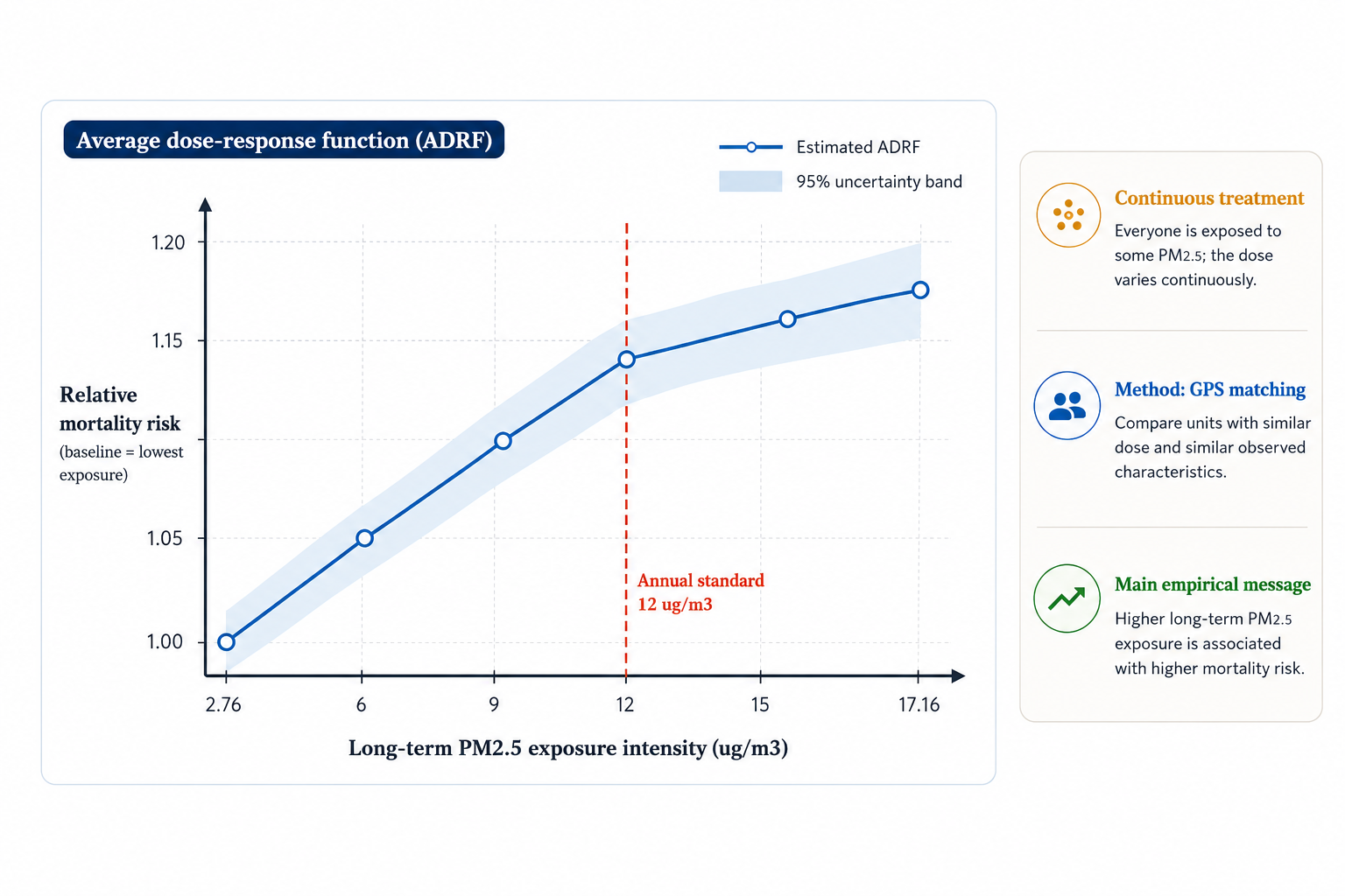
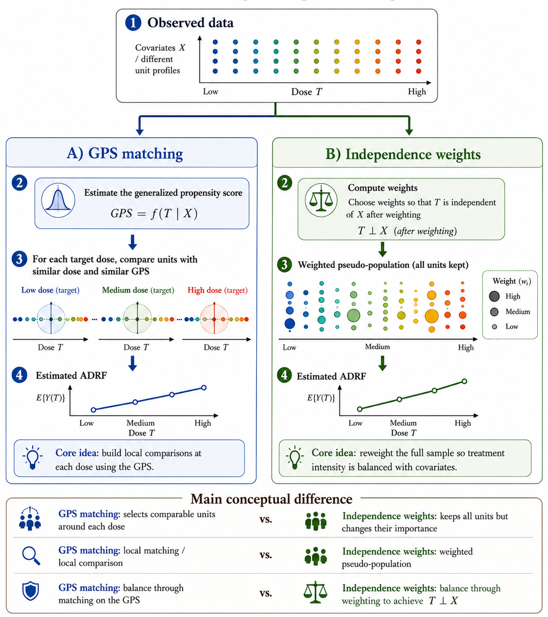
Wu et al. (2024) propose a matching approach for continuous treatments based on the GPS. This differs from the classical GPS approach of Hirano and Imbens, where the GPS is typically included as an adjustment variable in an outcome model to estimate the ADRF. In Wu et al.’s approach, the GPS is used more directly to construct matched comparisons among units with similar exposure levels and similar GPS values. The goal is to preserve the design-based intuition of matching while extending it beyond the binary treatment setting.
Their application studies the causal relationship between long-term exposure to fine particulate matter, PM\(_{2.5}\), and all-cause mortality among Medicare enrollees in the United States. Here, the treatment is not whether a unit is exposed to pollution, since everyone is exposed to some level of air pollution. The treatment is instead the intensity of exposure, measured by annual average PM\(_{2.5}\).
The method first estimates the GPS. Units are then matched so that, across different pollution levels, the distribution of observed covariates becomes more comparable. This produces a matched dataset that can be used to estimate an ADRF.
In the empirical application, the authors use data on 68.5 million Medicare enrollees from 2000 to 2016. Matching substantially improves covariate balance. The estimated exposure-response function shows that long-term PM\(_{2.5}\) exposure increases mortality, with evidence of adverse effects even at pollution levels below the national standard.
14.8 Beyond the Standard GPS
The GPS approach is powerful, but it relies on modeling choices that may be restrictive. Researchers must specify a treatment model and an outcome model. If these models are misspecified, the estimated ADRF may be biased.
Recent work has developed methods that focus more directly on balancing covariates across treatment intensities. One example is entropy balancing for continuous treatments (Tübbicke 2022). Another is the use of independence weights, which aim to make the treatment independent of observed covariates after weighting (Huling et al. 2024).
The common idea is to reduce dependence between treatment intensity and pre-treatment covariates without relying entirely on a parametric model for the treatment assignment process.
These approaches are part of a broader movement toward more flexible methods for continuous treatments. However, they do not remove the core identification problem. If important confounders are unobserved, weighting and balancing methods cannot recover the causal dose-response function by themselves.
14.9 Diagnostics and Validity Checks
A continuous-treatment analysis should report more than the estimated ADRF.
Inspect the distribution of treatment intensity. If most observations are concentrated in a narrow range, the dose-response function outside that range will have limited empirical support and rely heavily on extrapolation.
Assess common support. The analysis should show whether comparable units exist at different treatment levels.
Check covariate balance across the treatment distribution. The goal is to reduce the association between treatment intensity and pre-treatment covariates.
Report the ADRF with uncertainty bands. The curve may look smooth, but estimates at extreme treatment levels may be very imprecise.
Test sensitivity to alternative specifications. Researchers should assess robustness to alternative treatment models, outcome models, and dose ranges.
Before interpreting the shape of the ADRF, check whether the data actually contain comparable units observed at several different levels of treatment intensity.
14.10 Common Mistakes
Do not convert a continuous treatment into a binary treatment without a substantive reason. This may hide important variation in the relationship between treatment intensity and the outcome.
Do not interpret a raw regression of outcomes on treatment intensity as causal. In observational studies, units receiving different doses may differ systematically in their potential outcomes.
Do not estimate the dose-response function in regions with limited empirical support. This may turn heavy extrapolation into seemingly causal evidence.
Do not focus only on whether the curve is increasing or decreasing without considering uncertainty. Apparent nonlinearities may simply reflect statistical noise.
Do not ignore the relevant policy margin. The key question is often not the effect of moving from zero to a very high dose, but the effect of changing treatment intensity within the range over which policymakers can realistically intervene.
14.11 Worked Example
Suppose a government provides public subsidies to firms to reduce workplace accidents. A binary analysis would compare firms that receive a subsidy with firms that do not.
But the policy may provide different subsidy amounts. Some firms receive a small grant for basic safety equipment. Others receive a larger grant for major workplace redesign. A continuous-treatment analysis would ask how accident rates change as subsidy intensity increases.
Let \(T_i\) be the subsidy amount per worker. The ADRF is
\[ \mu(t)=E[Y_i(t)], \]
where \(Y_i(t)\) is the accident rate that firm \(i\) would have under subsidy intensity \(t\).
If the ADRF declines sharply at low subsidy levels and then flattens, this suggests that modest subsidies may generate most of the safety gains. If the function continues to decline at higher doses, larger subsidies may be justified. If the curve becomes flat or even increases, additional funding may be inefficient.
The credibility of this analysis depends on whether firms receiving different subsidy amounts are comparable after conditioning on pre-treatment characteristics such as firm size, sector, baseline accident rate, investment capacity, and previous safety inspections.
A single ADRF summarizes how the outcome changes with treatment intensity for the average unit. This may be misleading when units respond differently to the same dose. In that case, the pooled ADRF can hide subgroup-specific dose-response relationships, especially when common support is limited across groups.
A useful alternative is to estimate dose-response functions separately for theoretically defined or data-driven subgroups, as in the Clustered Dose-Response Function approach (Cerqua et al. 2026). The target then shifts from one population-average curve to a set of subgroup-specific curves, which may be more informative for policy design. However, creating more homogeneous groups does not automatically make the unconfoundedness assumption less demanding. Within each subgroup, treatment intensity may still be related to unobserved determinants of the outcome. A causal interpretation therefore still requires a credible justification for unconfoundedness and sufficient overlap over the doses being compared.
14.12 Summary
Continuous-treatment methods extend causal inference from the question of whether a unit is treated to the question of how much treatment it receives.
The main object of interest is the ADRF, which describes how expected outcomes change across treatment intensities. This is especially useful when policymakers need to decide not only whether to implement a policy, but also how intensely to implement it.
The main difficulty is that treatment intensity is rarely randomly assigned. Units receiving different doses may differ systematically. Methods such as the GPS and newer balancing approaches can help address selection on observed covariates, but they require strong assumptions and careful diagnostics.
Several software packages can be used to estimate effects with continuous treatments.
- R
CausalGPS: implements matching and weighting methods based on the generalized propensity score for continuous exposures.independenceWeights: implements independence weights for causal inference with continuous treatments.WeightIt: estimates balancing weights for binary, multi-valued, and continuous treatments.
- Python
causal-curve: estimates causal dose-response curves for continuous treatments.
- Stata
doseresponse: estimates the generalized propensity score, checks balance, and estimates dose-response functions.