5 Selection-on-observables methods
Selection-on-observables methods rely on the idea that treatment assignment is not random, but that all characteristics influencing both treatment assignment and potential outcomes are observed in the data. This means that, although treated and untreated units may initially differ, we assume that these differences can be accounted for using observed characteristics. If all relevant confounders1 are observed and measured before treatment, we can use these characteristics to construct a credible comparison between treated and untreated units. The underlying assumption is that, among units with the same relevant characteristics, treatment assignment is as good as random. The two main selection-on-observables approaches are regression adjustment and matching. Regression adjustment uses a statistical model to account for differences in observed pre-treatment characteristics between treated and untreated units, whereas matching constructs a comparison group by selecting untreated units with characteristics similar to those of the treated units. Both approaches therefore rely on the same central assumption: after conditioning on observables2, no unobserved confounders remain that affect both treatment assignment and potential outcomes.
1 A confounder is a variable that influences both whether a unit receives treatment and the outcome it would experience. Failing to account for confounders can lead us to attribute differences in outcomes to the treatment when they are actually due to pre-existing differences between treated and untreated units.
2 Conditioning on observables means accounting for observed characteristics so that the comparison is made between units with the same or similar values of these characteristics.
5.1 The linear regression model
The linear regression model is probably the most prominent tool in statistics and econometrics. In its simplest form, it describes the relationship between an outcome variable and one explanatory variable. In causal inference, this same tool can be used to estimate treatment effects, but only under specific assumptions. Dozens of excellent textbooks explain linear regression in detail, covering its statistical foundations, estimation, inference, diagnostics, and extensions. This chapter does not aim to provide a full treatment of the model. Instead, it focuses on its role in causal inference when embedded in the counterfactual approach. The key question is not only how to estimate a regression coefficient, but under what conditions that coefficient can be interpreted as a causal effect.
Suppose we observe a post-treatment outcome \(Y_i\) and a binary treatment indicator \(D_i\), where \(D_i=1\) for treated units and \(D_i=0\) for untreated units. A simple regression model can be written as
\[ Y_i = \alpha + \tau D_i + u_i. \]
In this model, \(\alpha\) is the average outcome for untreated units, while \(\tau\) captures the difference in average observed outcomes between treated and untreated units. The term \(u_i\) is the error term: it captures all factors affecting the outcome that are not included in the regression.3
3 Despite its name, the error term is not itself an error; rather, it represents the component of the outcome that is not explained by the variables included in the regression model.
The parameters \(\alpha\) and \(\tau\) are usually estimated by ordinary least squares (OLS), a statistical method widely used to estimate the parameters of regression models. In simple terms, OLS chooses the values of \(\alpha\) and \(\tau\) that minimize the sum of squared differences between observed and predicted outcomes. These differences are called residuals. In this way, OLS finds the parameter values that provide the best fit to the observed data according to this criterion.
With a binary treatment (\(D_i\)) and an intercept (\(\alpha\)), the OLS estimate of \(\tau\) is equal to the difference in sample means between treated and untreated units:
\[ \widehat{\tau}_{OLS} = \bar{Y}_{D=1} - \bar{Y}_{D=0}. \]
At the population level, this corresponds to
\[ \tau = E[Y_i \mid D_i=1] - E[Y_i \mid D_i=0]. \]
This coefficient is simply the difference in mean outcomes between treated and untreated units. In other words, it coincides with the difference-in-means (DIM) estimator introduced in previous chapters. This comparison has a causal interpretation if the average outcome of untreated units provides a credible estimate of what treated units would have experienced without treatment. In a properly implemented RCT with full compliance, random assignment ensures that this condition holds in expectation. Therefore, this simple regression can be used to estimate the ATE/ATT.
In observational studies, treated and untreated units often differ in characteristics that also affect their outcomes. As a result, the regression coefficient \(\tau\) does not generally isolate the causal effect of treatment. Recall that, as discussed in previous chapters, the DIM estimator combines the ATT with selection bias. Since the regression coefficient coincides with the DIM estimator, it suffers from the same problem: it may reflect both the causal effect of treatment and systematic pre-existing differences between the two groups.
For this reason, simple regression is rarely enough to identify causal effects in observational settings. A more useful starting point is the multiple regression model:
\[ Y_i = \alpha + \tau D_i + X_i'\beta + u_i, \]
where \(X_i\) is a vector of observed pre-treatment covariates. Ideally, these covariates should include all confounders, that is, all pre-treatment variables that affect both treatment assignment and potential outcomes.
The timing of the variables is crucial. The covariates in \(X_i\) must be measured before treatment occurs because we want to account for pre-existing differences between treated and untreated units, not differences that arise as a consequence of treatment. Controlling for variables that are themselves affected by treatment may distort the estimated treatment effect and prevent us from identifying the causal effect of interest. The outcome \(Y_i\), by contrast, must be measured after treatment to capture its potential effects.
In this model, \(\tau\) compares treated and untreated units holding constant the covariates included in \(X_i\).4 The idea is that, after adjusting for relevant observed pre-treatment differences, the remaining difference in post-treatment outcomes may provide a credible estimate of the ATT. For this interpretation to hold, several conditions are required.
4 Note that \(\tau\) in this model is generally different from the coefficient \(\tau\) in the simple regression model introduced above: the former accounts for differences in observed characteristics, whereas the latter captures the unadjusted difference in mean outcomes between treated and untreated units.
Covariates must be measured before treatment occurs.
There must be sufficient overlap (also known as common support) between treated and untreated units, meaning that for each treated unit there should be untreated units with similar values of the observed covariates. Without common support, the regression relies on extrapolation rather than on comparisons between similar units, making the estimated treatment effect more dependent on the assumed functional form of the regression model.5
The regression specification must be credible. OLS regression is a parametric adjustment method6: it specifies how the expected outcome varies with the covariates. If the assumed functional form is too restrictive, for example because it ignores important nonlinearities or interactions, the estimated treatment effect may be misleading. Suppose, for instance, that the outcome increases sharply with income only above a certain threshold. Including income as a simple linear term may fail to adequately account for income-related differences between treated and untreated units, potentially leading to a biased estimate of the ATT.
All relevant confounders must be observed and adequately controlled for. The key identifying assumption underlying both regression adjustment and matching methods is the conditional independence assumption (CIA), also known as unconfoundedness or selection on observables. It states that, conditional on the observed pre-treatment covariates \(X_i\), treatment status is independent of untreated potential outcomes: \[ Y_i(0) \perp D_i \mid X_i.\]
5 Extrapolation means using the estimated regression relationship to predict outcomes for units whose covariate values are not well represented in the comparison group. These predictions are more model-dependent because they are based on combinations of characteristics for which little or no comparable data are observed.
6 A method is called parametric when it assumes a specific functional form for the relationship between variables, described by a finite set of parameters to be estimated. For example, a simple linear regression assumes that a one-unit increase in a covariate is associated with a constant change in the expected outcome.
This means that, among units with the same observed characteristics, the average outcome of untreated units provides a credible estimate of what treated units would have experienced without treatment. If, however, a variable affects both selection into treatment and the outcome but is omitted from the regression model, this assumption may be violated and the OLS estimate may be biased. This is known as omitted variable bias.
Suppose we want to estimate whether installing speed cameras reduces the number of road accidents. The unit of analysis is a road segment. The treatment variable \(D_i\) is equal to 1 if road segment \(i\) receives a speed camera, and 0 otherwise. The outcome \(Y_i\) is the number of accidents observed after the installation period.
A first approach would be to estimate a simple regression model:
\[ Y_i = \alpha + \tau D_i + u_i. \]
In this model, \(\tau\) is simply the difference in average post-treatment accidents between roads with speed cameras and roads without speed cameras. This comparison would probably be misleading. Speed cameras are often installed on roads that were already more dangerous before the policy. These roads may have higher traffic volume, higher previous accident rates, different speed limits, or a different urban location.
For this reason, we may add observed pre-treatment characteristics to the model:
\[ Y_i = \alpha + \tau D_i + \beta_1 \text{Accidents}_{i,\text{pre}} + \beta_2 \text{Traffic}_{i,\text{pre}} + \beta_3 \text{SpeedLimit}_{i,\text{pre}} + X_i'\gamma + u_i, \]
where \(X_i\) may include other pre-treatment characteristics, such as road type, urban density, weather exposure, or nearby intersections. These controls are included because they may affect both the probability that a speed camera is installed and the outcome of interest, namely the number of road accidents.
In the latter model, \(\tau\) compares road segments with and without speed cameras holding constant these observed pre-treatment characteristics. The counterfactual logic is the following: for a treated road segment, the regression uses information from untreated road segments with similar characteristics to estimate how many accidents would have occurred without the camera.
The expression “holding constant” can be misleading when treated and untreated units are very different in their pre-treatment characteristics. In some applications, there may be no untreated units that are comparable to the treated ones for relevant values of \(X_i\).
For example, suppose speed cameras are installed only on particularly dangerous roads with high pre-treatment accident rates and heavy traffic. If no untreated roads have similar characteristics, the regression model must extrapolate from roads that are quite different to estimate the counterfactual outcome. OLS can still produce an estimate of \(\tau\), but this estimate may depend heavily on the assumed linear functional form rather than on comparisons between comparable treated and untreated units.
In this case, although the regression formally holds the observed covariates constant, the data provide little or no direct evidence about what would have happened to the treated roads without speed cameras. This is a problem of lack of common support, which we will discuss in more detail in the section on matching.
Ultimately, it is important to remember that OLS regression is not inherently causal. It becomes a tool for causal inference only when embedded in a credible research design and supported by appropriate identifying assumptions, which are often quite demanding. Without a credible justification for these assumptions, the estimated treatment coefficient captures a conditional association rather than a causal effect. In the next section, we introduce matching methods, which address the same problem of selection on observables through a different strategy: rather than relying on a regression model to adjust for differences between units, they explicitly construct a comparison group of untreated units with characteristics similar to those of the treated units.
5.2 Matching Methods
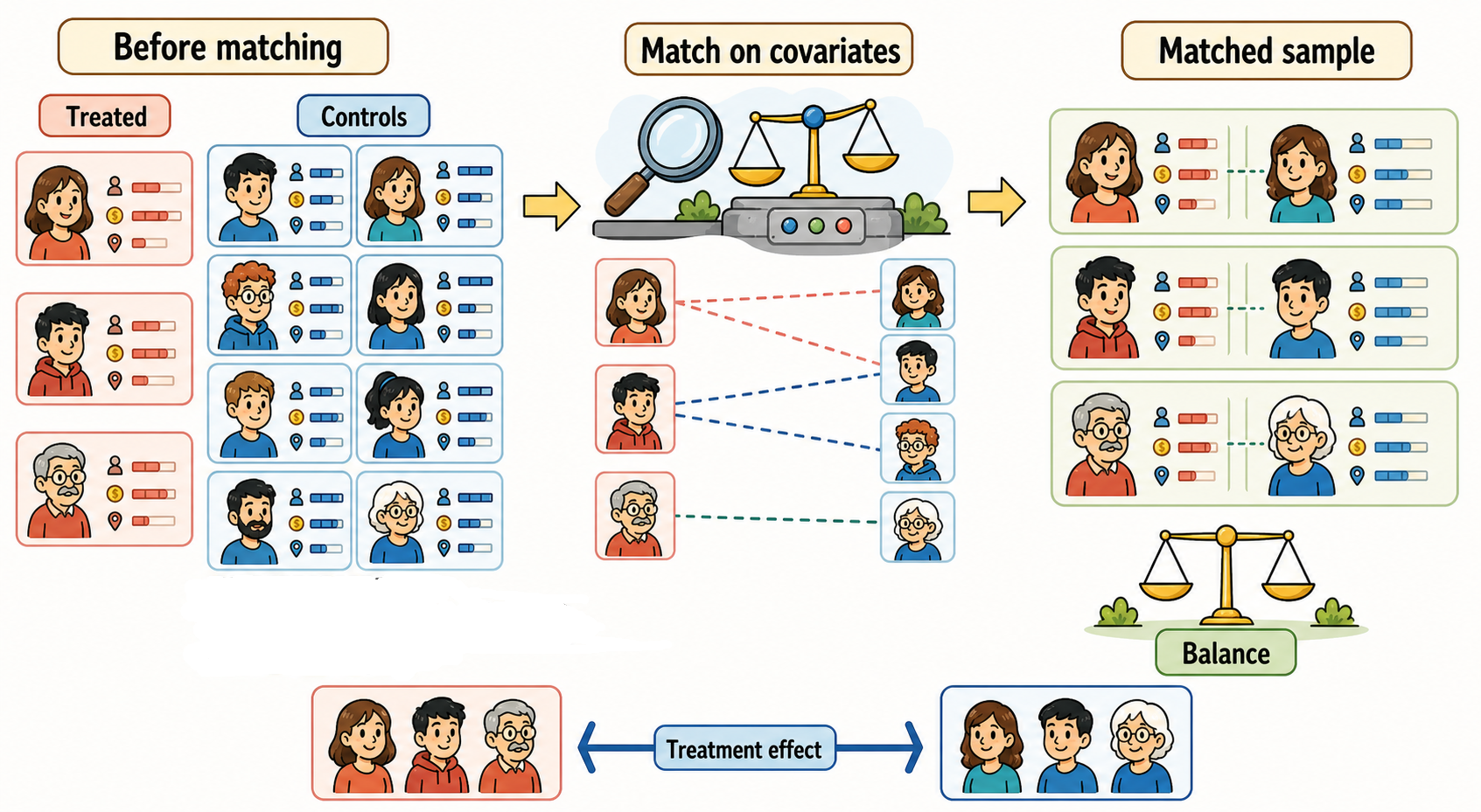
The idea behind matching methods is simple: after treatment assignment has occurred, the control group is constructed ex post by selecting untreated units that are similar to treated units in terms of observed pre-treatment characteristics. These matched untreated units are then used to approximate the counterfactual outcomes that treated units would have experienced in the absence of treatment. Unlike in an RCT, therefore, comparability is not created by randomization but by the matching procedure.
Suppose we want to evaluate the effect of a policy \(D_i\) on an outcome \(Y_i\). As usual, each unit has two potential outcomes: \[ Y_i(1) \quad \text{and} \quad Y_i(0).\]
We are interested in the ATT:
\[ ATT = E[Y_i(1)\mid D_i=1] - E[Y_i(0)\mid D_i=1]. \]
The first term is observed: \[ E[Y_i(1)\mid D_i=1] = E[Y_i^{obs}\mid D_i=1].\]
The second term is not observed. It is the average outcome that treated units would have experienced without treatment. Matching methods estimate this missing counterfactual by selecting untreated units whose observed pre-treatment characteristics are as similar as possible to those of the treated units.
5.2.1 The Logic of Matching
In an observational study, treatment is not randomly assigned. Units may select into treatment, or policymakers may select units for treatment, based on characteristics that also affect the outcome. Matching tries to make treated and untreated units comparable after the data have been collected. It does so by comparing treated units only with untreated units that have similar values of observed covariates \(X_i\).
For example, suppose we want to estimate the effect of an after-school tutoring program on students’ test scores. Students who attend the program may differ from non-participants in previous achievement, family background, motivation, teacher recommendations, or school attendance. Matching would compare each participating student with one or more non-participating students who are similar in terms of the observed pre-treatment variables.
Matching replaces the impossible comparison between treated units and their own missing counterfactual outcomes with a comparison between treated units and untreated units with similar observed pre-treatment characteristics.
5.2.2 Historical Intuition
The early intuition behind matching was close to the logic of experimental blocking. In an experiment, units may be grouped into blocks with similar characteristics before randomization. Matching applies a related idea to observational data: since treatment was not randomly assigned, the researcher tries to restore comparability by pairing or grouping treated and untreated units with similar pre-treatment characteristics.
Early work focused on relatively direct forms of adjustment. One approach was subclassification, where units were divided into groups based on one or more covariates and comparisons were made within those groups. Cochran (1968) showed how subclassification could remove a large share of bias when the covariate used for adjustment was strongly related to selection into treatment and the outcome.
Rubin’s early work developed the logic of matched sampling more explicitly within the potential outcomes framework. The key idea was that a good matched comparison should make the distribution of pre-treatment covariates similar across treated and untreated groups, so that the remaining difference in outcomes could be interpreted more plausibly as a treatment effect (Rubin 1973a, 1973b). Cochran and Rubin (1973) also reviewed how matching, subclassification, and regression adjustment could be used to reduce bias in observational studies.
5.2.3 Conditional Independence Assumption
As mentioned above, matching relies on a key identifying assumption: the CIA, i.e., \[ Y_i(0) \perp D_i \mid X_i.\]
Under this assumption,
\[ E[Y_i(0)\mid D_i=1, X_i=x] = E[Y_i(0)\mid D_i=0, X_i=x]. \]
In other words, treated and untreated units with the same observed characteristics would have experienced the same outcome, on average, in the absence of treatment.
The key difference is that we cannot observe \(Y_i(0)\) for treated units, whereas we can observe it for untreated units:
\[ Y_i^{obs}=Y_i(0) \quad \text{when } D_i=0. \]
Therefore, by matching treated units with untreated units that have similar pre-treatment characteristics, we can use the observed outcomes of the latter to estimate what the treated units would have experienced, on average, without treatment.
Importantly, this assumption cannot be fully tested. What we can check is whether the matching process improved balance between the two groups, making them similar on average in terms of observed pre-treatment characteristics.
This is a crucial limitation of matching: it can account only for differences in observed characteristics. Suppose that treated and untreated units differ in characteristics that are not observed in the data, such as motivation, ability, managerial quality, or political connections. If these characteristics also influence the outcome, even units that appear very similar based on observed variables may differ systematically in their potential outcomes. As a result, matching may fail to eliminate selection bias.
Matching can adjust for differences in observed pre-treatment characteristics.
It cannot remove bias due to unobserved variables that affect both treatment assignment and the outcome.
5.2.4 Common Support
For the estimation of the ATT, a second key assumption is common support, also called overlap. For each relevant value of the covariates, there must be at least one untreated unit similar to each of the treated ones.
Formally,
\[ P(D_i=1\mid X_i=x) < 1. \]
This condition means that, for units with characteristics \(X_i=x\), treatment is not certain. In other words, among units with the same, or sufficiently similar, observed characteristics, there must be some untreated units that can serve as comparisons for the treated units. If the probability of receiving treatment is equal to one for a given set of characteristics, matching cannot construct a credible counterfactual for treated units with those characteristics.
In practice, lack of common support means that some treated units cannot be matched with comparable untreated units. Excluding these treated units makes the remaining comparisons more credible, but it also changes the population to which the estimated treatment effect refers. For example, suppose firms of all sizes receive a subsidy, but large treated firms have no comparable untreated firms. We may then have to exclude large firms from the analysis. As a result, we would no longer estimate the ATT for all subsidized firms, but only for the subset of small and medium-sized subsidized firms for which comparable untreated firms exist.
Matching requires treated and untreated units to overlap in terms of observed pre-treatment covariates.
Units outside the common support should not be used for causal comparisons, because comparing units with substantially different characteristics may lead to biased estimates that reflect pre-existing differences rather than the causal effect of treatment.
5.2.5 Exact Matching
In the ideal case, each treated unit would be matched with one or more untreated units that have exactly the same values of the pre-treatment covariates.
Suppose \(X_i\) contains age, education, and previous earnings. Exact matching would compare a treated individual only with untreated individuals that have the same age, the same education level, and the same previous earnings.
The matching estimator for the ATT can be described in three steps:
- Divide the data into groups (also called strata or cells) defined by the values of \(X_i\).
- Within each stratum, compute the difference between the average post-treatment outcomes of treated and untreated units.
- Compute a weighted average of these differences, assigning to each stratum a weight equal to the proportion of all treated units that it contains.
The last step is important. Since the ATT measures the average effect across treated units, each treated unit should contribute equally to the estimate. Therefore, strata containing more treated units receive greater weight in the final estimate.
Formally, under the CIA and common support, the ATT can be written as
\[ ATT = E_X \left[ E(Y_i\mid D_i=1,X_i) - E(Y_i\mid D_i=0,X_i) \mid D_i=1 \right]. \]
This expression captures the core idea of matching: compare the average post-treatment outcomes of treated and untreated units with the same observed characteristics, and then average these differences over the treated population. The outer expectation is taken with respect to the distribution of \(X_i\) among treated units, so each treated unit contributes equally to the ATT.
For example, suppose we want to estimate the effect of a refresher training course on participants’ earnings. We perform exact matching using two binary pre-treatment covariates: whether the worker is young or older, and whether the worker lives in an urban or rural area.
This creates four covariate cells:
| Covariate cell | Treated workers | Mean earnings (€), treated | Mean earnings (€), untreated | Within-cell difference |
|---|---|---|---|---|
| Young, urban | 20 | 32 | 28 | 4 |
| Older, urban | 35 | 38 | 31 | 7 |
| Young, rural | 10 | 26 | 24 | 2 |
| Older, rural | 35 | 34 | 30 | 4 |
The ATT is not the simple average of the four within-cell differences. Averaging them mechanically would give 4.25 euros:
\[ \frac{4+7+2+4}{4}=4.25. \]
Instead, the ATT weights each cell by its share of treated units. Since there are 100 treated workers, the weights are 0.20, 0.35, 0.10, and 0.35:
\[ ATT = 0.20 \times 4 + 0.35 \times 7 + 0.10 \times 2 + 0.35 \times 4 = 4.85. \]
The reason is that the ATT asks: what is the average effect for the treated workers? Therefore, each treated worker receives the same weight. Cells with more treated workers contribute more to the final ATT estimate.
5.2.6 The Curse of Dimensionality
As the number of covariates in \(X_i\) increases, finding untreated units with exactly the same observed pre-treatment characteristics as treated units becomes increasingly difficult, or even impossible. With continuous covariates, exact matches may be extremely rare, and even when all covariates are binary, the number of possible covariate profiles grows rapidly as more variables are included. This problem is known as the curse of dimensionality.
For example, with 20 binary covariates, there are
\[ 2^{20} = 1{,}048{,}576 \]
possible combinations of covariate values, each defining a potential stratum.
This means that a very large dataset may be needed to find treated and untreated units within the same strata. In practice, this makes exact matching infeasible in many empirical applications.
5.2.7 Propensity Score Matching
An influential approach to addressing the curse of dimensionality is propensity score matching (PSM), introduced by Rosenbaum and Rubin (1983).
The propensity score is the probability of receiving the treatment conditional on observed covariates:
\[ p(X_i) = P(D_i=1\mid X_i). \]
This probability is not directly observed. What we observe is whether each unit actually received the treatment or not. However, before treatment occurs, we can think of each unit as having some underlying probability of receiving the treatment, depending on its observed characteristics. The propensity score represents this probability and must generally be estimated from the data, for example using a logit or probit model (see below). The resulting estimated propensity score is denoted by \(\widehat{p}(X_i)\). Instead of matching units on all the individual covariates in \(X_i\), PSM matches them on a single number: their estimated propensity score.
Rosenbaum and Rubin showed that the propensity score is a balancing score: conditional on its true value7, treated and untreated units have the same distribution of observed covariates:
7 The true value refers to the actual probability of receiving treatment given the observed characteristics, \(p(X_i)\), rather than its estimate, \(\widehat{p}(X_i)\), obtained from a statistical model.
\[ X_i \perp D_i \mid p(X_i). \]
This is known as the balancing property of the propensity score. However, this property guarantees balance only in observed covariates, not in unobserved characteristics.
They also showed that, if treatment assignment is independent of potential outcomes conditional on \(X_i\), this independence also holds conditional on the propensity score:
\[ (Y_i(1),Y_i(0)) \perp D_i \mid X_i \quad \Rightarrow \quad (Y_i(1),Y_i(0)) \perp D_i \mid p(X_i). \]
This result has an important implication: instead of comparing units with the same values of all observed covariates, we can compare units with the same propensity score. For these comparisons to be possible, however, we also need sufficient overlap in the propensity score distributions of treated and untreated units.
In practice, the true propensity score is unknown and must be estimated from the data. Therefore, we should always check whether matching on the estimated propensity score achieves adequate balance in observed covariates.
The propensity score reduces a multidimensional matching problem to a one-dimensional one. Instead of matching on many covariates, we match units on a single number: their estimated probability of receiving treatment.
5.2.7.1 Estimating the Propensity Score
In practice, the true propensity score is unknown and must be estimated. This is usually done by modelling treatment assignment as a function of pre-treatment covariates.
Common choices include:
Linear probability model
\[ P(D_i=1\mid X_i)=\beta_0 + X_i'\beta. \]
Probit model
\[ P(D_i=1\mid X_i)=\Phi(\beta_0 + X_i'\beta). \]
Logit model
\[ P(D_i=1\mid X_i)= \frac{\exp(\beta_0+X_i'\beta)} {1+\exp(\beta_0+X_i'\beta)}. \]
In general, logit and probit models are preferred because they ensure that the estimated propensity scores, \(\widehat{p}(X_i)\), lie between 0 and 1.
The covariates included in \(X_i\) should be chosen carefully. They should be pre-treatment variables that affect treatment assignment and are plausibly related to the outcome. If panel data are available, lagged outcomes can often be useful because they capture pre-treatment differences in outcome levels.
5.2.7.2 Matching Rules
Once the propensity score has been estimated, we need to choose a criterion for matching treated and untreated units. In practice, propensity scores are usually continuous values between 0 and 1, often measured with many decimal places. For this reason, it is unlikely that one or more untreated units will have exactly the same propensity score as a treated unit.
In practice, for each treated unit, we select untreated units whose estimated propensity scores are sufficiently close to its own. Different matching methods determine how these comparison units are selected. Selecting only very similar units can help reduce bias, while including more comparison units can improve the precision of the estimate.
Matching rules differ in how they select and weight untreated units to construct the counterfactual for each treated unit, including the number of control units used. Selecting only the closest control units can reduce bias by ensuring that comparisons are made between units with very similar pre-treatment characteristics. However, relying on fewer control units may increase the variance of the estimate. Conversely, using more control units can improve precision but may increase bias if these additional units are less comparable to the treated unit.
The choice of matching rule therefore involves a bias–variance trade-off: closer matches tend to reduce bias, while using more comparison units tends to improve precision.
In what follows, we briefly discuss some of the most common matching rules.
Stratification matching. The range of the propensity score is divided into intervals, or strata. Within each stratum, treated and untreated units should have similar propensity scores. For example, we might divide units into five equally spaced strata based on their estimated propensity scores: 0–0.2, 0.2–0.4, 0.4–0.6, 0.6–0.8, and 0.8–1.
The treatment effect is estimated within each stratum as the difference in mean outcomes between treated and untreated units. These stratum-specific effects are then averaged, weighting by the number of treated units in each stratum.
If the data are divided into \(S\) strata (five in the example above), the ATT estimator can be written as
\[ \widehat{ATT}_{strat} = \sum_{s=1}^{S} \frac{N_{1s}}{N_1} \left( \overline{Y}_{1s} - \overline{Y}_{0s} \right), \]
where \(N_{1s}\) is the number of treated units in stratum \(s\), \(N_1\) is the total number of treated units, and \(\overline{Y}_{1s}\) and \(\overline{Y}_{0s}\) are the average post-treatment outcomes of treated and untreated units in that stratum.
One-nearest-neighbor matching. Each treated unit is matched to the untreated unit with the most similar propensity score.
For treated unit \(i\), the matched control is
\[ j(i) = \arg\min_{j:D_j=0} \left| \widehat p(X_i)-\widehat p(X_j) \right|. \]
The ATT is then estimated as the average difference between each treated unit and its matched control:
\[ \widehat{ATT}_{NN} = \frac{1}{N_1} \sum_{i:D_i=1} \left[ Y_i - Y_{j(i)} \right]. \]
Nearest neighbor matching can be implemented with or without replacement. With replacement, the same untreated unit can be used as a match for multiple treated units.8
8 Matching with replacement generally improves match quality because each treated unit can be matched with its closest untreated unit, even if that unit has already been used as a match. This can reduce bias but may increase variance, particularly when a small number of untreated units are repeatedly used to construct the counterfactuals for many treated units. In this case, the estimate relies heavily on the outcomes of a few control units.
A common extension is \(K\)-nearest-neighbor matching. Instead of selecting only the closest untreated unit, each treated unit is matched to the \(K\) closest untreated units, with common choices being \(K=3\) or \(K=5\). Increasing \(K\) can improve precision but may increase bias by including less comparable control units.
Radius matching. Each treated unit is matched to all untreated units whose propensity score lies within a fixed distance, or radius.
For treated unit \(i\), the set of matched controls contains all untreated units \(j\) such that
\[ D_j = 0 \quad \text{and} \quad \left| \widehat p(X_i)-\widehat p(X_j) \right| \le r. \]
Here, \(r\) is the radius, also referred to as the caliper.
The choice of \(r\) involves a trade-off. A smaller radius improves comparability but may leave some treated units unmatched. A larger radius increases the number of matches but may include poorer matches, increasing bias. There is no universal choice of \(r\): it should be selected based on the scale of the propensity score, the quality of overlap, and balance diagnostics.
Kernel matching. The counterfactual outcome for each treated unit is constructed as a weighted average of untreated outcomes. Untreated units with propensity scores closer to that of the treated unit receive larger weights, while more distant units receive smaller weights or may receive no weight.
The bandwidth determines how quickly weights decline as the distance in propensity scores increases.9
For treated unit \(i\), the counterfactual outcome is estimated as
\[ \widehat{Y}_i(0) = \sum_{j:D_j=0} w_{ij}Y_j, \]
where the weights \(w_{ij}\) depend on the distance between the propensity score of treated unit \(i\) and the propensity score of untreated unit \(j\).
The ATT is then
\[ \widehat{ATT}_{kernel} = \frac{1}{N_1} \sum_{i:D_i=1} \left[ Y_i - \widehat{Y}_i(0) \right]. \]
Kernel matching constructs the counterfactual for each treated unit as a weighted average of the outcomes of multiple untreated units, giving greater weight to those with more similar propensity scores. Unlike nearest-neighbor matching, kernel matching can use information from many untreated units. The choice of bandwidth is crucial: a smaller bandwidth concentrates the weights on more similar units, potentially reducing bias, while a larger bandwidth spreads the weights across more units, potentially improving precision.
9 In kernel matching, the bandwidth controls how broadly control units are used around each treated unit. A smaller bandwidth gives most weight to very close matches, while a larger bandwidth allows more distant controls to receive meaningful weight.
5.2.8 Other Matching Approaches
The matching methods discussed so far are part of a broader family of approaches that share a common goal: constructing credible comparison groups based on observed pre-treatment characteristics. They differ in how they define similarity between units, select and weight comparison units, and handle the trade-offs between transparency, flexibility, bias, and precision. The aim here is not to cover all matching methods in detail, but to introduce the main intuition and briefly mention a few additional approaches.
Mahalanobis matching matches units using a multivariate distance measure computed directly on the covariates. Unlike propensity score matching, which reduces the covariates to a single scalar, Mahalanobis matching compares units in the original covariate space. The Mahalanobis distance between two units is based on the difference in their covariate values, adjusted by the covariance matrix of the covariates.10 In this way, differences are standardized and correlations among covariates are taken into account. It can work well when the number of covariates is limited, but it becomes less practical as the number of covariates increases.
10 The covariance matrix summarizes both how much each covariate varies across units (its variance) and how different covariates vary together (their covariances).
Coarsened exact matching first transforms covariates into substantively meaningful categories, or bins. For example, age may be grouped into age bands (18–29, 30–49, 50–64), income into income brackets (below $20,000, $20,000–$50,000, above $50,000), and firm size into size classes (micro, small, medium, and large firms). Exact matching is then performed within these coarsened covariate cells. This approach is attractive because it is transparent: the researcher explicitly defines what counts as “similar.” The cost is that results may depend on how the covariates are coarsened.
Other related balancing approaches include genetic matching, full matching, and covariate balancing propensity score methods.
5.2.9 Reweighting methods
Propensity scores can also be used in a different way. Instead of matching treated and untreated units with similar propensity scores, reweighting methods use the propensity score to assign different weights to observations. The goal is to create a weighted comparison group that is balanced in terms of observed pre-treatment characteristics.
The most common approach is inverse probability weighting (IPW). The basic idea is simple: units that are unlikely to receive the treatment they actually received are given more weight, because they are especially informative for constructing the counterfactual comparison. The weights assigned to treated and untreated units depend on the causal estimand of interest.
To estimate the ATE, treated units are weighted by the inverse of their probability of receiving treatment, while untreated units are weighted by the inverse of their probability of remaining untreated:
\[ w_i^{ATE} = \frac{D_i}{p(X_i)} + \frac{1-D_i}{1-p(X_i)}, \]
where \(p(X_i)=P(D_i=1 \mid X_i)\) is the propensity score. The goal is to reweight both groups so that their distributions of observed characteristics resemble that of the overall population.
To estimate the ATT, instead, treated units receive a weight of 1, while untreated units are weighted by the ratio of their probability of receiving treatment to their probability of remaining untreated:
\[ w_i^{ATT} = D_i + (1-D_i)\frac{p(X_i)}{1-p(X_i)}. \]
In this case, the treated group remains unchanged, while the untreated group is reweighted to resemble the treated group in terms of observed pre-treatment characteristics.
In both cases, the treatment effect can be estimated by comparing the weighted average outcomes of the two groups. The key difference is the population that these weights aim to represent: the entire population for the ATE and the treated population for the ATT.
Reweighting methods are similar to PSM because they rely on the same identifying assumptions, namely conditional independence and overlap, and use the propensity score to make treated and untreated units comparable in terms of observed pre-treatment characteristics. The difference lies in how the comparison is constructed: PSM selects untreated units that are similar to treated units, while reweighting methods usually keep all observations but change their relative importance through weights. In this way, weighting constructs a weighted pseudo-population in which treatment assignment is balanced with respect to observed covariates, rather than selecting a limited set of matched controls.
A key limitation is that weighting can be sensitive to extreme propensity scores. For instance, when estimating the ATE, if some treated units have a very low probability of being treated (e.g., 0.02), or some untreated units have a very high probability of being treated (e.g., 0.98), their weights can become very large (50 in both cases). When estimating the ATT, extreme weights arise only among untreated units with very high propensity scores (e.g., a propensity score of 0.98 results in a weight of 49). For this reason, checking overlap and inspecting the distribution of weights are essential diagnostic steps.
In short, PSM and reweighting methods share the same counterfactual logic: they seek to make treated and untreated groups comparable in terms of observed pre-treatment characteristics. They differ, however, in how they achieve this goal.
- Matching asks: Which untreated units should we select to construct a credible comparison group?
- Weighting asks: How much weight should each unit receive to make the groups comparable?
5.2.10 Assessing Match Quality
Estimating the ATT is not the final step of a matching analysis. We must also assess whether matching has achieved its main objective: making the distributions of observed pre-treatment covariates as similar as possible between treated and matched untreated units. This step is known as covariate balance assessment.
Common diagnostics include:
- comparing covariate means before and after matching;
- checking standardized mean differences between treated and matched untreated units for relevant pre-treatment covariates;
- inspecting the distribution of the propensity score;
- verifying common support;
- reporting how many treated and untreated units are unmatched or discarded.
The credibility of an ATT estimate obtained through matching depends on two important conditions: sufficient common support, so that treated units have comparable untreated units, and adequate covariate balance, so that treated and matched control units are similar in terms of their observed pre-treatment characteristics. Importantly, even when both conditions are satisfied, a causal interpretation still requires the CIA to hold.
Before interpreting the estimated treatment effect, check whether matching has achieved adequate covariate balance. If substantial imbalances remain, the matched comparison group may not provide a credible counterfactual.
5.2.11 What Bias Does Matching Remove?
Matching can address two important sources of bias. To illustrate them, consider a setting in which the ATT is the causal estimand of interest:
Lack of common support. Matching can exclude treated units for which no comparable untreated units exist, avoiding potentially misleading comparisons between units with substantially different characteristics.
Covariate imbalance. Matching can select and weight untreated units so that the distribution of their observed pre-treatment characteristics becomes more similar to that of the treated units.
However, matching cannot eliminate bias arising from selection on unobservables.11 Even after achieving good balance in observed covariates, treated and matched untreated units may still differ systematically in these unobserved characteristics, leading to biased estimates of the ATT.
11 Selection on unobservables occurs when characteristics that are not observed in the data influence both treatment assignment and potential outcomes. For example, firms with more capable managers may be more likely to apply for a subsidy and perform better even without the subsidy.
In other words, matching can help with bias due to observed differences between treated and untreated units, but not with bias due to unobserved differences.
Matching can improve the comparability of treated and untreated units with respect to observed pre-treatment characteristics. However, it cannot balance factors that are unobserved. Therefore, matching identifies a causal effect only if, after conditioning on the observed covariates, there are no remaining unobserved factors that jointly affect treatment assignment and potential outcomes.
5.2.12 Empirical Illustration
An example of matching in applied research is the study by Bovan et al. (2018) on the effect of natural disasters on voting behavior. The authors study whether voters punish politicians for events outside their control, focusing on floods in Croatia.
Flooded and non-flooded areas may differ systematically. For example, they may differ in socioeconomic conditions, geography, political preferences, or previous voting behavior. A simple comparison between flooded and non-flooded areas may therefore be misleading.
The study uses one-nearest-neighbor matching to compare affected and non-affected areas with similar observed characteristics. The balancing table below illustrates the logic of the procedure. Before matching, flooded municipalities differed substantially from non-flooded municipalities in several pre-treatment characteristics. After matching, these differences became much smaller.
| Variable | Flooded | Non-flooded, before matching | Absolute difference before matching | Non-flooded, after matching | Absolute difference after matching | ||
|---|---|---|---|---|---|---|---|
| Unemployment | 23.46 | 17.34 | 6.12 | 22.98 | 0.48 | ||
| \(\rule{0pt}{0.2em}\) | |||||||
| Income per capita | 19,237.45 | 22,471.44 | 3,233.99 | 19,299.04 | 61.59 | ||
| \(\rule{0pt}{0.2em}\) | |||||||
| Municipal income per capita | 1,340.43 | 2,220.85 | 880.42 | 1,196.84 | 143.59 | ||
| \(\rule{0pt}{0.2em}\) | |||||||
| Education | 63.23 | 70.56 | 7.33 | 63.63 | 0.40 |
Before matching, floods appeared to reduce support for incumbent politicians. After accounting for differences in control variables through matching, the estimated flood effect disappeared.
This example illustrates the core logic of matching: part of what looks like a treatment effect may actually reflect pre-existing differences between treated and untreated units. Matching tries to reduce this problem by constructing a comparison group that is more similar to the treated group in terms of observed pre-treatment characteristics.
5.3 Matching vs. Regression Adjustment
Matching methods and regression adjustment are closely related. Both try to make treated and untreated units comparable in terms of pre-treatment characteristics. They differ mainly in how they use the covariates.
Matching methods first construct a comparison group. Treated units are compared with untreated units that have similar values of the relevant pre-treatment covariates. The adjustment is therefore made by choosing which control units are used in the comparison and how much weight each receives.
Regression adjustment, instead, uses all available observations and relies on a statistical model to account for differences in covariates between treated and untreated units. The adjustment is therefore made by modeling how the expected outcome varies with the observed pre-treatment characteristics, allowing us to compare treated and untreated units while holding these characteristics constant.
The two approaches can also be combined. A common strategy is to first match treated and untreated units to improve covariate balance, and then estimate a regression model on the matched sample. In this case, matching reduces the dependence on functional-form assumptions, while regression adjustment can improve precision and correct remaining small imbalances.
The key difference is that matching is more transparent about the comparison being made: it shows which untreated units are used to approximate the counterfactual outcomes of treated units, whether there is sufficient common support, and how well the observed covariates are balanced after matching. Regression adjustment, by contrast, is more model-based: it relies more heavily on the assumed relationship between covariates and outcomes, and may conceal problems of limited overlap or poor covariate balance.
They also differ in how they handle failures of common support. With matching, lack of overlap is usually visible: treated units without comparable untreated units cannot be matched, or are matched only poorly. These units may then be excluded from the analysis, changing the population for which the effect is estimated. With regression adjustment, by contrast, the model can still estimate counterfactual outcomes for treated units outside the support of the control group, but doing so requires extrapolation and makes the ATT estimate much more dependent on functional-form assumptions.
5.4 Summary
Regression adjustment and matching methods estimate causal effects by accounting for differences in observed pre-treatment characteristics between treated and untreated units. They are especially useful when treatment is not randomly assigned but rich pre-treatment information is available.
The key assumptions are:
- Conditional Independence Assumption: after conditioning on observed covariates, treatment assignment is as good as random.
- Common support: treated units have comparable untreated units.
The two approaches differ in how they adjust for pre-existing differences. Regression adjustment models the relationship between covariates and outcomes, whereas matching constructs a comparison group by selecting and weighting untreated units with characteristics similar to those of treated units.
Matching is particularly attractive because it is intuitive, makes the comparison between units explicit, and facilitates the assessment of common support and covariate balance. Regression adjustment, by contrast, relies more heavily on the assumed functional form of the outcome model.
The main limitation of both approaches is their reliance on selection on observables. If important unobserved factors affect both treatment assignment and potential outcomes, neither regression adjustment nor matching alone can solve the identification problem.
Several software packages can be used to implement matching methods.
- R
- Python
- Stata