11 Forecast-Based Counterfactual Methods
The methods discussed so far rely on the availability of untreated units that can be used to construct a credible counterfactual. However, in many policy settings, such units may be unavailable or may not provide a credible comparison group. For instance, this may occur when:
The treatment affects all units at the same time. This can happen with nationwide reforms, macroeconomic shocks, pandemics, or policies implemented simultaneously across all units. In such settings, no untreated units may remain in the data.
Untreated units are indirectly affected by the treatment. This may happen when a policy changes labor-market conditions, prices, commuting flows, local competition, or social interactions. In such cases, untreated units no longer represent what would have happened to treated units in the absence of the policy, because they are themselves affected by it. This violates the no-interference assumption (Cox 1958).
In these cases, control-based evaluation strategies cannot be leveraged to recover the causal effects of interest. To overcome such a limitation, a possible solution would be to use evaluation strategies that do not rely on the post-treatment values of the untreated units to recover the causal estimands of interest. In particular, in this chapter, we will focus on forecast-based counterfactual methods (FBCMs), namely methods that leverage pre-treatment information to forecast the counterfactual scenario of each treated unit.
The logic is simple: if no credible control group is available, we can use the pre-treatment information of the treated units themselves to forecast the missing counterfactual.1
1 In some settings, pre-treatment information from untreated units can also be used to improve the forecast, even if those units cannot provide a credible post-treatment comparison group.
FBCMs estimate what would have happened after the intervention by projecting the pre-treatment behavior of the treated units into the post-treatment period.
This approach estimates causal effects by comparing the observed post-treatment outcomes of the treated units with the outcomes forecasted for the same units in the absence of the treatment, using only their pre-treatment data. The counterfactual is therefore constructed through a forecasting model rather than through a comparison with untreated units.
11.1 The Evaluation Problem
For simplicity, we focus on the case of a single treated unit, but the same reasoning extends to settings with multiple treated units. Consider a unit observed over time. Let \(t=1,\ldots,T_0\) denote the pre-treatment period and \(t=T_0+1,\ldots,T\) denote the post-treatment period. The intervention starts after \(T_0\).
For each post-treatment period, the observed outcome is
\[ Y_t^{obs}=Y_t(1), \]
while the missing counterfactual is \(Y_t(0)\).
The individual treatment effect (ITE) at time \(t\) is
\[ \tau_t = Y_t(1) - Y_t(0), \qquad t > T_0. \]
Since \(Y_t(0)\) is not observed after the intervention, FBCMs replace it with a prediction:
\[ \widehat{\tau}_t = Y_t^{obs}-\widehat{Y}_t(0). \]
The crucial step is therefore the construction of \(\widehat{Y}_t(0)\).
11.2 Counterfactual Forecasting
The construction of the counterfactual can be seen as a prediction problem (Varian 2014, 2016). FBCMs use pre-treatment information to predict what the post-treatment outcome would have been in the absence of treatment.
In its most compact form, a forecast-based estimator can be written as
\[ \widehat{Y}_t(0)=\widehat{f}(\mathcal{H}_{T_0}), \]
where \(\mathcal{H}_{T_0}\) is the information available before treatment. This information may include pre-treatment values of the outcome and other covariates, time-invariant characteristics, seasonal patterns, and underlying trends.
The treatment effect is then the gap between the observed post-treatment outcome and the predicted untreated path.
The logic is intuitive: the pre-treatment evolution of the outcome is used to predict what would have happened after treatment in its absence. Any systematic departure from this predicted path can then be interpreted as evidence of a treatment effect, provided the forecasting assumptions are credible (see Section 11.7).
For example, suppose employment in a country had been increasing steadily before a reform. If employment rises substantially more than predicted after the reform, the additional increase may be attributed to the treatment. A similar logic is used to measure excess mortality. During a pandemic, for instance, mortality observed in a region can be compared with the baseline level predicted from pre-pandemic data; the difference is interpreted as excess mortality.
However, this difference can be interpreted causally only if the forecasted counterfactual is credible.
FBCMs replace cross-sectional comparison with time-series prediction. This avoids the need for untreated units, but it requires a set of different assumptions about the stability and predictability of the untreated outcome path.
11.3 Simple Forecasting Methods
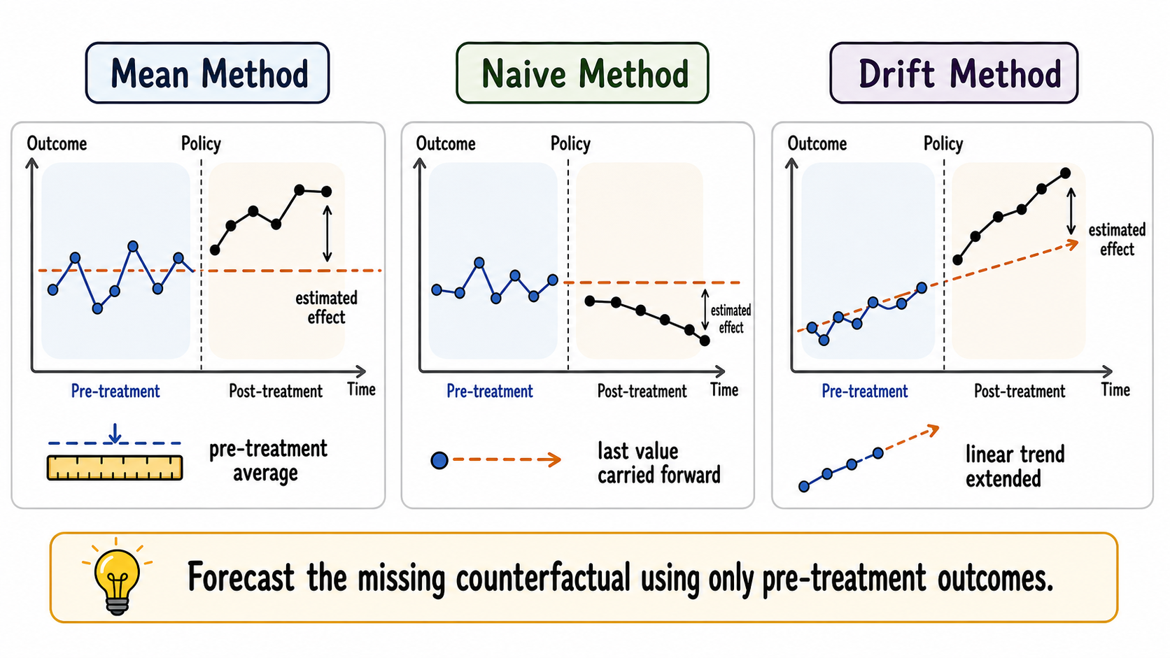
A first family of methods uses very simple forecasting methods. These methods are useful because they make the core intuition of FBCMs transparent.
Simple forecasting rules are rarely enough for a final evaluation, but they are useful benchmarks. A more sophisticated method should usually improve on them in pre-treatment placebo forecasting exercises.
11.3.1 Mean Method
The mean method uses the average pre-treatment outcome as the counterfactual forecast:
\[ \widehat{Y}_{T_0+h}(0)=\frac{1}{T_0}\sum_{t=1}^{T_0}Y_t. \]
This approach is reasonable only if the untreated outcome is approximately stable over time. It is often too crude when there are trends, cycles, or seasonality.
The report by the Italian National Social Security Institute (INPS 2020) on mortality during the Covid-19 epidemic provides a useful example of a mean-method counterfactual. To assess excess mortality in early 2020, the report compares observed deaths with a baseline given by the average number of deaths in the same calendar period of previous years.
This approach is credible in this application because all-cause mortality is relatively stable over short periods once seasonality is taken into account. Excess mortality is then estimated as the difference between observed deaths in 2020 and this historical mean baseline.
11.3.2 Naive Method
The naive method uses the last pre-treatment observation as the forecast:
\[ \widehat{Y}_{T_0+h}(0)=Y_{T_0}. \]
This can be useful when the best short-run prediction is the most recent value. But it fails when outcomes were already trending before the intervention.
11.3.3 Drift Method
The drift method extends the pre-treatment trend linearly:
\[ \widehat{Y}_{T_0+h}(0)=Y_{T_0}+h\frac{Y_{T_0}-Y_1}{T_0-1}. \]
This method allows for a linear trend, but it remains simplistic. If the untreated outcome follows nonlinear dynamics, seasonal patterns, or sudden changes unrelated to the policy, the forecast may be inaccurate.
11.4 From Forecast Error to Treatment Effect
Once a counterfactual forecast is available, several causal parameters can be constructed.
The point effect at post-treatment time \(t\), with \(t > T_0\) is
\[ \widehat{\tau}_t=Y_t^{obs}-\widehat{Y}_t(0). \]
The cumulative effect up to period \(T\) is
\[ \widehat{\Delta}_T=\sum_{s=T_0+1}^{T}\widehat{\tau}_s. \]
The temporal average effect is
\[ \widehat{\bar{\tau}}_T= \frac{1}{T-T_0}\sum_{s=T_0+1}^{T}\widehat{\tau}_s. \]
With several treated units, the researcher can also average across units:
\[ \widehat{ATT}_t= \frac{1}{N}\sum_{i=1}^{N} \left(Y_{it}^{obs}-\widehat{Y}_{it}(0)\right). \]
The same logic can also be used to study treatment-effect heterogeneity by comparing the estimated effects across different subgroups of treated units.
11.5 Interrupted Time-Series Design
An interrupted time-series design compares the observed post-intervention outcome with the continuation of the pre-intervention time-series pattern.
The interrupted time-series (ITS) design is probably the most widely used FBCM. It is particularly useful when there is a single treated unit and a sufficiently long pre-treatment time series is available to model its underlying trajectory.
The idea is to model the pre-treatment dynamics of the outcome and then extrapolate them into the post-treatment period.
A simple ITS model can be written as
\[ Y_t=\alpha+\beta t+\gamma Post_t+\delta(t-T_0-1)Post_t+u_t, \]
where \(T_0\) denotes the last pre-treatment period and \(Post_t=\mathbf{1}(t>T_0)\). The intervention therefore starts at \(T_0+1\). In this specification, \(\beta\) captures the pre-intervention trend, \(\gamma\) captures the immediate level change relative to the counterfactual trend in the first treated period, and \(\delta\) captures the change in trend after the intervention. The term \((t-T_0-1)Post_t\) equals zero in the first treated period, so the intervention-related change at that point is \(\gamma\). Thereafter, the post-intervention trend is \(\beta+\delta\).
This representation is useful pedagogically, but real applications often require more careful modeling. Outcomes may be autocorrelated, seasonal, volatile, or affected by calendar effects. For this reason, ITS analysis is often combined with time-series models such as ARIMA.
The counterfactual is the predicted path that would have occurred after \(T_0\) if the pre-treatment dynamics had continued without the intervention.
The ITS design works best when the number of pre-treatment periods is large. With few pre-treatment observations, it is difficult to learn the untreated dynamics, distinguish signal from noise, and assess whether the post-treatment deviation reflects a genuine treatment effect rather than random fluctuations.
11.5.1 Application: the Italian smoking ban
In January 2005, Italy introduced a regulation banning smoking in indoor public places. Suppose we want to study whether this policy reduced hospital admissions for acute coronary events, as in Cesaroni et al. (2008). Importantly, the smoking ban was introduced nationally, and all Italian regions were exposed to the policy at the same time.
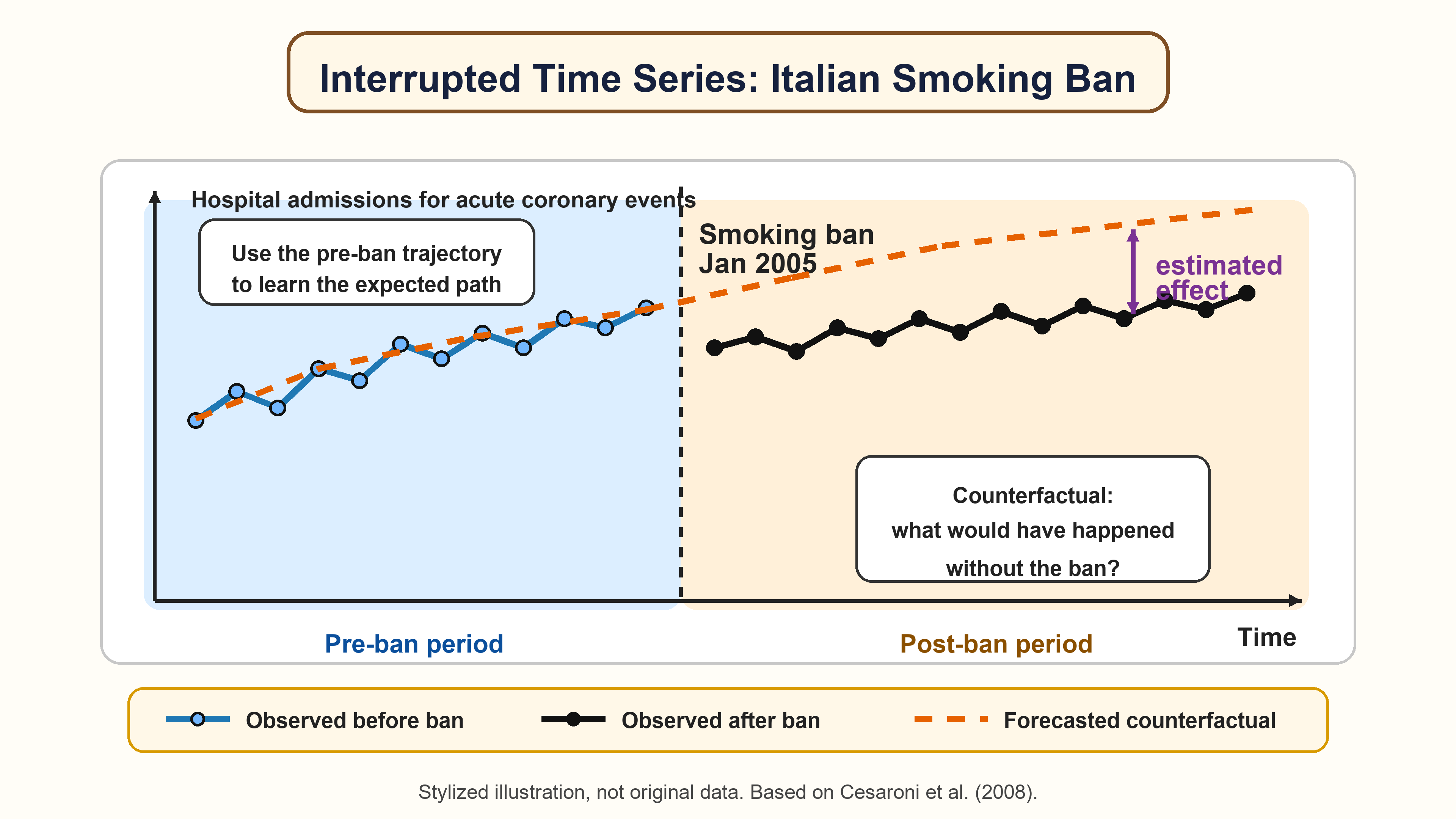
Since all units in Italy were treated simultaneously, there is no obvious untreated group within the country that can be used to construct the counterfactual. One possibility would be to use similar data from other countries that did not introduce the same policy at the same time. However, this strategy would be credible only if other countries provided a suitable comparison for Italy and hospital admission data were measured in a sufficiently comparable way across countries.
For this reason, an ITS design offers a natural alternative. Instead of relying on untreated units, this approach uses a model that exploits the pre-policy trajectory of hospital admissions in Italy to forecast what would have happened after January 2005 in the absence of the smoking ban.
If post-ban admissions fall below what would have been expected from the pre-ban trend (as in the figure above), this difference can be interpreted as evidence consistent with a positive policy effect, provided that the forecasted counterfactual is credible and that no other simultaneous event explains the change.
11.5.2 Causal-ARIMA
Causal-ARIMA extends the ITS logic by explicitly anchoring ARIMA models in the potential outcomes framework (Menchetti et al. 2023). It is designed for settings in which no control series is available and the researcher has a sufficiently long pre-treatment time series.
The key contribution is not simply the use of ARIMA as a forecasting method. Rather, the method embeds forecasting within a causal framework: it defines causal estimands using potential outcomes, clarifies the assumptions under which deviations from the forecast can be interpreted as treatment effects, and provides a framework for statistical inference.
The basic idea can be summarized in four steps:
- estimate the untreated time-series process using pre-treatment data;
- forecast how the outcome would have evolved after treatment in its absence;
- compare the observed post-treatment outcomes with this forecast to estimate treatment effects;
- quantify the uncertainty surrounding these estimates.
For example, Causal-ARIMA has been used by (Menchetti et al. 2023) to estimate the effect of a permanent price reduction on sales in a retail setting where only the treated product series is available. The treatment effect is estimated as the difference between observed post-treatment sales and the sales that would have been predicted in the absence of the price reduction.
A confidence interval describes the uncertainty around an estimated parameter or expected outcome, such as an average treatment effect. It asks: how precisely have we estimated the quantity of interest?
A prediction interval describes the uncertainty around an individual future or unobserved outcome. It accounts not only for uncertainty in the estimated model, but also for the variability of the outcome around its predicted mean. It asks: how uncertain is the outcome we are trying to predict?
This distinction is particularly relevant for counterfactual methods. In CBCMs, such as DiD or matching, the main object is usually a causal parameter obtained by comparing treated units with observed control units. Inference therefore typically focuses on uncertainty around the estimated treatment effect, which is reported using confidence intervals.
In FBCMs, the counterfactual is forecast from the treated unit’s own pre-treatment history rather than observed in a comparison group. If the object of interest is the specific counterfactual outcome that would have occurred, uncertainty concerns an unobserved outcome itself, making a prediction interval a natural inferential object. If instead the object of interest is the expected counterfactual outcome or an average treatment effect, confidence intervals may also be appropriate.
11.6 Machine Learning Control Method
The Machine Learning Control Method (MLCM) generalizes the forecast-based logic to richer panel settings with many treated units and no credible control group (Cerqua et al. 2024).
The central idea is to use supervised machine learning algorithms, such as LASSO, random forests, and gradient boosting, to learn how outcomes evolve in the absence of treatment using only pre-treatment information. The model is then used to predict post-treatment counterfactual outcomes for treated units.
In this framework, a generic counterfactual forecast can be written as
\[ \widehat{Y}_{it}(0)=\widehat{f}(X_i,\mathcal{H}_{i,T_0},t), \]
where \(X_i\) denotes pre-treatment characteristics and \(\mathcal{H}_{i,T_0}\) denotes the pre-treatment history of unit \(i\).
Compared with simple time-series methods, MLCM can exploit many predictors and flexible nonlinear relationships. It is particularly useful when the researcher observes many treated units, such as municipalities, firms, or schools, but cannot rely on untreated units as controls.
Cerqua, Letta, and Menchetti (2024) apply the MLCM to study the impact of the COVID-19 shock on educational achievement in Italy. This is a natural setting for the MLCM because the shock affected the whole country at the same time: there is no obvious untreated control group that can be used to construct the counterfactual.
The units of analysis are Italian Local Labor Markets. The outcome is the standardized INVALSI mathematics test score of fifth-grade students. The authors use a rich set of pre-COVID predictors, including past INVALSI scores, local socioeconomic conditions, demographic characteristics, labor-market indicators, and territorial features, to forecast what each local area’s math score would have been in the absence of the pandemic. The difference between the observed post-shock score and the machine-learning forecast gives the estimated local treatment effect.
The results show a large negative effect of the COVID-19 shock on learning outcomes, averaging about -0.76 standard deviations relative to the forecasted counterfactual. Losses are uneven across space and are larger in already fragile areas, especially those with higher unemployment, higher inequality, and lower educational attainment.
11.7 Identification Assumptions
FBCMs require a set of assumptions that is almost completely different from those used in control-group designs.
Stability of the untreated outcome process. In the absence of treatment, the relationship learned from pre-treatment data should continue to hold in the post-treatment period. If the data-generating process changes for reasons unrelated to the policy, the forecast error may capture those changes rather than the treatment effect.
Absence of other simultaneous shocks. If another event that could itself affect the treated units’ outcome occurs at the same time as the treatment, it may be impossible to disentangle the effect of the treatment from that of the concurrent event.
- Sufficient pre-treatment information. Forecasting requires enough historical data to learn the relevant pattern.2
2 There is no universal minimum number of pre-treatment periods. What counts as enough depends on the complexity and stability of the outcome process: learning trends, seasonality, or other recurring patterns generally requires a longer pre-treatment series than learning a simple and stable trajectory.
- No anticipation. Units should not change behavior before the start of the intervention because they expect the treatment to occur. Anticipation contaminates the pre-treatment period and makes the estimated untreated trajectory unreliable. This assumption also underlies most CBCMs.
Machine learning, time-series models, or a combination of the two can improve the accuracy of the counterfactual forecast, but accurate prediction alone is not enough for causal inference. If another event affects the treated units’ outcome after treatment, the observed deviation from the forecast may partly reflect this event rather than the treatment effect of interest.
11.8 Diagnostics and Validation
Because these methods rely heavily on prediction, validation is central.
A useful diagnostic is a pre-treatment forecasting exercise. The researcher can pretend that treatment occurred earlier, estimate the model using only data before that placebo date, and test how well the method predicts the held-out pre-treatment observations.
Before interpreting a post-treatment gap as a causal effect, ask whether the method would have predicted the pre-treatment path reasonably well.
If the model cannot predict the pre-treatment period, it is difficult to trust its post-treatment counterfactual forecast.
Other useful checks include:
- inspecting forecast errors during the pre-treatment period;
- comparing the placebo performance of the chosen method with simple forecasting benchmarks, such as the mean, naive, and drift methods;
- checking whether the results are driven by a few influential periods;
- examining whether other shocks occurred around the intervention date.
A promising recent development is the emergence of tabular foundation models, such as TabPFN and TabFM. Unlike conventional forecasting algorithms, these models are pretrained across millions of synthetic datasets and can transfer what they have learned to a new prediction problem through in-context learning, often without task-specific training or extensive hyperparameter tuning.
This feature is particularly relevant when the available dataset is not large. TabPFN has shown strong predictive performance on small and medium-sized tabular datasets, including regression problems with relatively few observations (Hollmann et al. 2025). TabPFN-TS extends this approach to forecasting by transforming time-series information into a tabular regression problem. Recent evidence indicates that it can produce competitive forecasts even without time-series-specific pretraining (Hoo et al. 2026). Newer models such as TabFM further develop this zero-shot approach for tabular regression and classification.
These advances could represent an important step forward for FBCMs. Policy evaluations often have only a limited number of pre-treatment periods or observations, but may contain many informative predictors. A pretrained foundation model could exploit complex relationships among these predictors more effectively than a model trained from scratch on the application dataset.
However, it is important to keep in mind that, although tabular foundation models may substantially strengthen the forecasting component of FBCMs, they do not replace the assumptions required for causal identification.
11.9 Worked Example
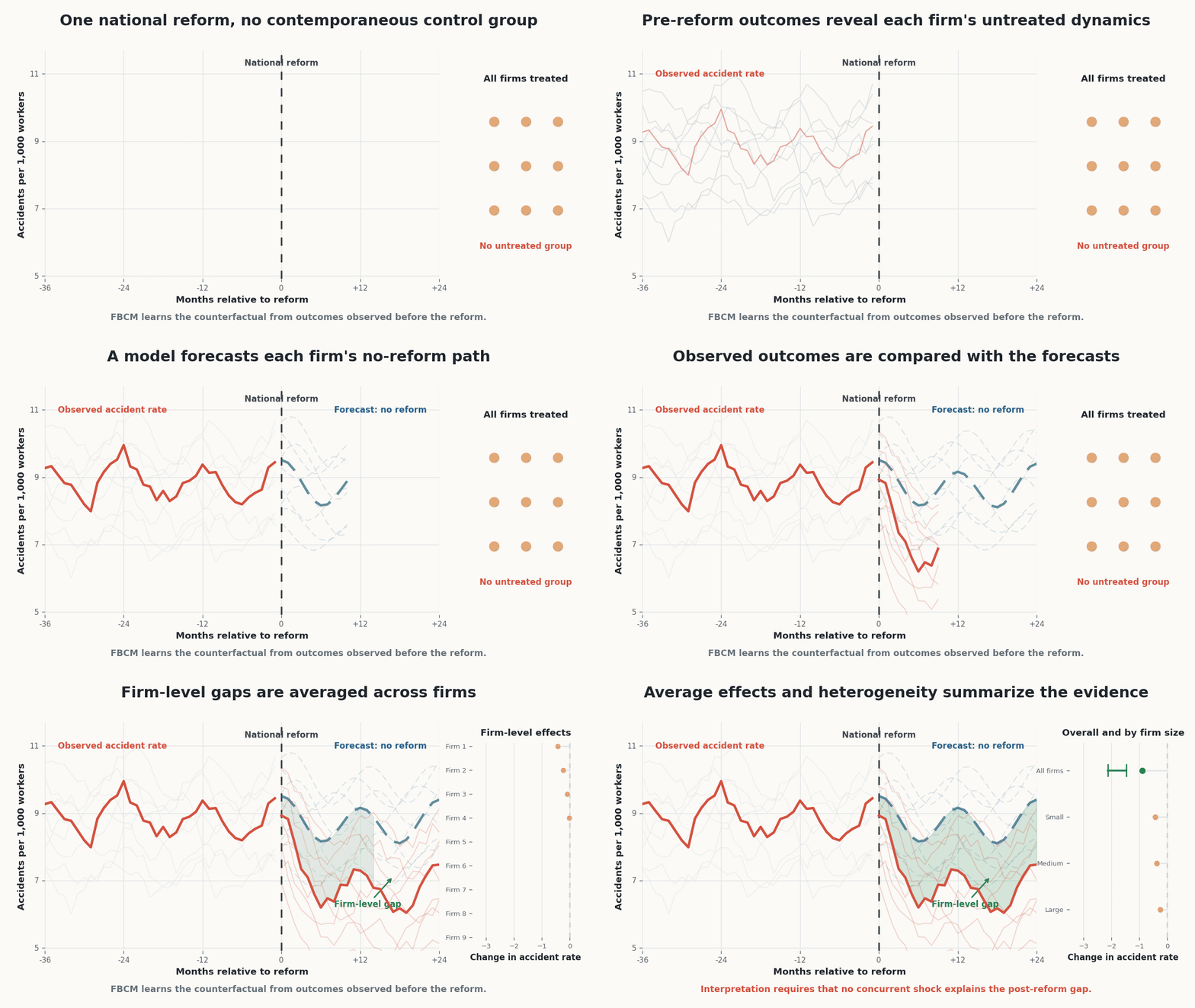
Suppose a national reform introduces a new workplace-safety regulation for all firms at the same time. The goal is to reduce workplace accidents. Because the reform is implemented nationwide, there is no contemporaneous untreated group of comparable firms within the country.
For each firm, we observe monthly accident rates for several years before the reform and after the reform. A FBCM would proceed as follows:
- Use pre-reform accident rates to model the expected accident path in the absence of the new regulation.
- Forecast the post-reform counterfactual accident rate.
- Compare observed post-reform accident rates with the predicted no-reform path.
- Average the estimated firm-level gaps to obtain the average treatment effect, and then compute the associated uncertainty.
- Examine whether the effect differs by firm size, sector, or baseline accident risk.
If observed accidents fall below the predicted counterfactual path after the reform, this is consistent with a beneficial effect. But the interpretation depends on whether other factors changed at the same time, such as new enforcement rules, reporting requirements, or macroeconomic conditions.
A controlled interrupted time-series (controlled ITS) design combines elements of forecast-based and control-based counterfactual methods. As in a standard ITS, the pre-intervention trajectory of the treated series is used to project how its outcome would have evolved after the intervention. At the same time, one or more untreated series are used to capture contemporaneous shocks or changes that are unrelated to the intervention.
The causal effect is therefore inferred from whether the treated series changes at the intervention date relative to both its own previous trajectory and the change observed in the control series. Compared with an uncontrolled ITS, this can make the counterfactual more credible when treated and control series would have been affected similarly by other events occurring during the study period (Lopez Bernal et al. 2018).
This advantage depends on the choice of controls. The control series should have comparable pre-intervention dynamics, should be exposed to the same relevant external shocks, and should not itself be affected by the intervention. A poorly chosen control can weaken rather than strengthen the design.
11.10 Summary
FBCMs provide a valuable alternative to CBCMs, especially when no credible control group exists. Instead of comparing treated and untreated units, they compare observed post-treatment outcomes with predicted untreated outcomes.
The simplest versions use mean, naive, or drift forecasts. More sophisticated approaches include ITS designs and the MLCM.
The strength of these methods is that they can be applied in settings where standard comparison-based methods fail, especially when no credible untreated group is available. Their weakness is that causal interpretation relies heavily on the credibility of the forecasted counterfactual. The key question is therefore whether the model can accurately learn the untreated outcome dynamics from pre-treatment data and extrapolate them into the post-treatment period.